Mod5 Unsupervised and Supervised Classification

This module introduces and explores both unsupervised and supervised classification methods. Unsupervised classification utilizes an algorithm to determine which pixels in the raster image are most like other pixels throughout the image and groups them based on a defined accuracy percentage. After the software has grouped the various pixels together it is up to the user to define what the grouped classes represent. For this type of classification the software is given certain user defined parameters such as number of iterations to run, confidence or threshold percentage to reach, and sample sizes. These essentially tell the software how long to run, what the minimum "correctly grouped" pixel percentage is, and how many pixels to look at adjusting at a time. 

On the other hand, supervised classification utilized user created training sites to tell the software what to look for spectrally to garner the user desired classifications. This is accomplished by creating a polygon area or a software grown similarity region. Examples would be forest, grassland, or water. Each area has a distinct spectral signature. These signatures are used to evaluate the whole of the image and allow the software to automatically reclassify all matching spectral signatures. The overall process is usually in 4 steps, get your image, establish spectral signatures, run the classification based on the signatures, then reclassify or identify rather what your class schema is.

Lets look at the two different areas that were used for the unsupervised and supervised processes respectively. 

This is not a refined map, but a screenshot from the software itself highlight an unsupervised classification output that has been recoded from 50 classes down to 5 specific classifications. This is the UWF campus which was originally a true color image whose pixel data has been reclassified. 

This is a complete map for the supervised classification portion of the module, centered on Germantown Maryland. It was created using a base image and supervised classification looking for the categories displayed in the legend. This map shows the acreage of areas as they currently exist and is intended to provide a baseline for change. As areas get developed the same techniques can be used on more and more current imagery to map the change and gauge which land uses are expanding / shrinking most and by how much.

Thank you.

v/r

Brandon

Mod 4, Spatial Enhancement and Spectral Analysis

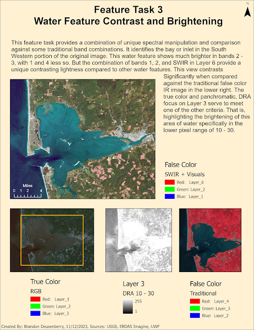
  This week's topic revolved around multi-spectral analysis through spectral enhancement. This involved taking existing spectral data and presenting it in a manner that might bring out certain relationships or patterns that might not have been originally obvious. The objective was to study an image set and identify certain spectral relationships by evaluating information available across multiple bands of the same image. Manipulating the pixel values through particular enhancements, and then identifying specific values correlating to specific feature types in the image helped build confidence in both ERDAS Imagine and ArcGIS. Both tools were used to explore the given image. Several tools within ERDAS were used, such as the Inquire cursor to look at particular groups of pixels for their relevant brightness information. Histograms and contrast information were used to identify patterns within multi-spectral and panchromatic views of one or more spectral bands. Specific criteria were provided for us to evaluate the image and locate features that matched. The first criteria involved locating features that correlate to a spike in the histogram data within spectral band 4  in values between 12 and 18.

The second criteria involved locating the feature that represents both a spike in the visual and NIR bands with a value around 200, and a large spike in the infrared layers of bands 5 and 6 around pixel values 9 to 11.

The last criteria being looked for revolves around water features that when looking at bands 1-3 become brighter than usual, but remain relatively constant in bands 5 and 6.

All three of the above maps with their specific different feature identifications relied upon the same general scheme of evaluation. First, the criteria were examined against the different bands histograms for the corresponding feature spike. Then a series of dynamic range adjustments between the bands was used to highlight specific pixel values. Then after the features were located, a set of bands were used to highlight the corresponding feature. Note that all of the main map images themselves are presented with a different band combination. Then the insets have some commonality amongst them to help give context to the main features. 

Thanks for stopping by,

V/r

Brandon

Module 3, Intro to ERDAS Imagine, and Thematic Mapper Classification

 ERDAS Imagine is another one of the primary softwares that we are using within this course. This week was an intro to it, and a look at some practical uses with Landsat Thematic Mapper imagery. Along with the basic ERDAS functionality, I looked into pre-processing an image within on software, then compiling a useable map within another, ArcGIS Pro in this case. 

The imagery software was used to organize and display a pre-classified image. In this case, the subject area is in the Olympic National Park area of Washington State. I chose the Mt. Lawson region and derived a subset image from a broader view of the park. The software was used to identify the area in hectares associated with all of the different classification types. Additionally, there were several themes explored while working with this and other images. Specifically looking at how spectral, spatial, and temporal resolution all work with different image types, and even multispectral images allowing for multi-band presentations. 

 While the above is a relatively simplistic map, the majority of the exploration for this weeks lab was within the ERDAS software itself. Additionally, there was an emphasis on understanding wavelength, frequency, and energy, associated with different portions of the electromagnetic spectrum. A couple key takeaways for this work were that the shorter the wavelength, the higher the frequency. The greater the frequency, the greater the energy. 

I look forward to moving into understanding how to do this type of image classification with the software and working to better incorporate multispectral imagery. Thank you for coming along with me.

v/r

Brandon